Welcome to Project Lovelace! We're still in early development so there are still tons of bugs to find and improvements to make.
If you have any suggestions, complaints, or comments please let us know on Discourse, Discord, or GitHub!
Let's look at an example of chaos arising from simplicity in nature: the logistic map. It's a simplified model used to
describe population sizes and can be written mathematically as
$$ x_{n+1} = rx_n(1 - x_n) $$
where $0 < r < 4$ is a parameter and $0 < x_n < 1$ represents the population size at time step $n$. Starting with an
initial population size of $x_0 = 0.5$ and $r$ as an input parameter, return a list of the first 50 values of the
logistic map $x_0, x_1, x_2, \dots, x_{49}, x_{50}$. You should see different behavior depending on the value of $r$,
but we'll leave you to play around with it and we'll have more to say in the solution notes.
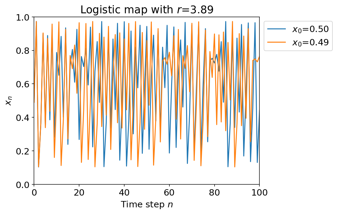
Logistic map with $r=3.89$ using two initial conditions ($x_0=0.50$ and $x_0=0.49$). It shows two big features of
chaotic systems. (1) It's sensitive to initial conditions as the two solutions start close to each other but quickly
diverge and look completely different after just several iterations. (2) The solutions don't really repeat so
they're nonperiodic which also means it's hard to predict them. (Plot generation code is in the solution notes.)
Input:
The parameter $r$.
Output:
A list containing the first 51 values of the logistic map $(x_0, x_1, x_2, \dots, x_{49}, x_{50})$.
The sensitivity to initial conditions exhibited by the logistic map is more commonly known as the butterfly effect. It means that unless you knew
the initial conditions exactly, there will be uncertainty in future predictions and is why we can only predict the
weather up to roughly two weeks ahead (much less in many cases).
If you plot the value the logistic map ends up at for each value of $r$ you get a bifurcation diagram for
the logistic map, which matches
up beautifully with the Mandelbrot set if you're into that sort of thing.
The logistic map was first introduced as a simple model of population dynamics with very complicated dynamics.
Let us know what you think about this problem! Was it too hard? Difficult to understand? Also feel free to
discuss the problem, ask questions, and post cool stuff on Discourse. You should be able see a discussion
thread below. Would be nice if you don't post solutions in there but if you do then please organize and
document your code well so others can learn from it.